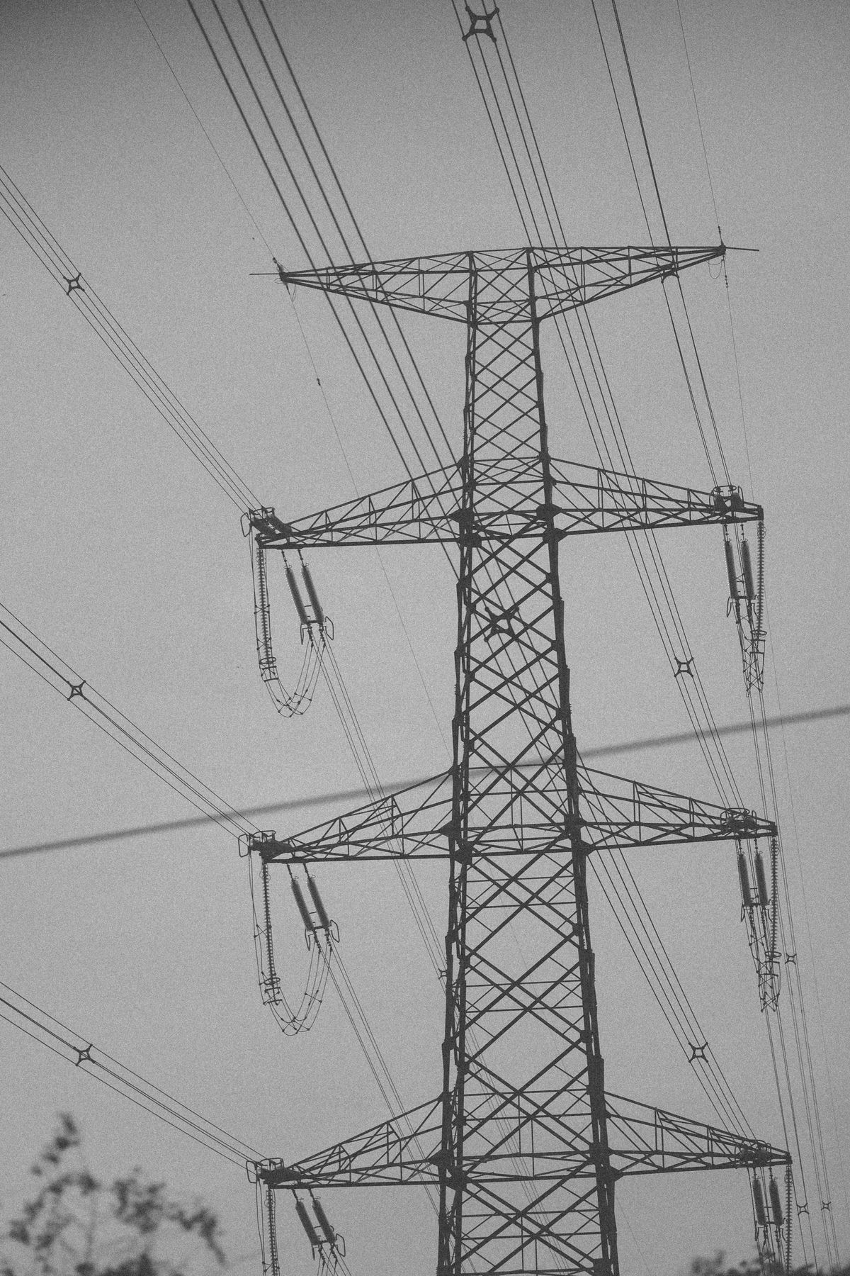
Low Voltage Network Distribution: Engineering Principles, Design Methodology, and System Optimization for Modern Power Networks

Figure 1: Low voltage distribution networks form the critical final stage between medium voltage substations and end consumers.
---
1. Introduction: The Engineering Significance of LV Distribution
Low voltage (LV) network distribution represents the final and most complex stage of the electrical power delivery system. While transmission and sub-transmission networks operate at tens or hundreds of kilovolts and serve relatively predictable bulk loads, LV networks operate at voltages ≤1000 V AC (IEC 60364) or ≤600 V AC (NEC Article 240), serving highly diverse, stochastic, and dynamically changing loads. The engineering challenge of LV distribution lies not in the magnitude of power transferred but in the complexity of managing voltage regulation, power quality, protection coordination, load balancing, and economic optimization across thousands of feeders serving millions of connection points.
The technical definition of "low voltage" varies by standard. IEC 60038 defines LV as voltages between 50 V and 1000 V AC (or 75–1500 V DC). The NEC defines LV as ≤600 V. Common nominal LV distribution voltages worldwide include 230/400 V (50 Hz systems, Europe, most of Asia, Africa), 120/240 V (60 Hz, North America split-phase), 127/220 V (some Latin American countries), and 220/380 V (transitional systems). The choice of nominal voltage has cascading implications for conductor sizing, voltage drop calculations, short-circuit current levels, protection device selection, and transformer sizing — making voltage selection the first and most consequential design decision in LV network planning.
---
2. Topological Configurations of LV Networks
2.1 Radial Topology
The radial configuration is the most common LV network topology worldwide due to its simplicity and cost-effectiveness. Power flows unidirectionally from the MV/LV transformer to the load points through a tree-like structure of main feeders and laterals. The key engineering relationship governing radial feeder design is the voltage drop equation:
$$\Delta V = \frac{P \cdot R + Q \cdot X}{V_n} \cdot L$$
Where:
- $\Delta V$ = voltage drop (V)
- $P$ = active power flow (W)
- $Q$ = reactive power flow (var)
- $R$ = resistance per unit length (Ω/km)
- $X$ = reactance per unit length (Ω/km)
- $V_n$ = nominal voltage (V)
- $L$ = feeder length (km)
The percentage voltage drop must comply with regulatory limits — typically ±5% or ±6% of nominal voltage at the point of supply, and ±10% at the point of utilization (EN 50160 for European systems). For a 230 V system, this means the maximum allowable drop from the transformer secondary to the furthest consumer is approximately 23 V (10%), requiring careful conductor sizing and feeder length management.
2.2 Ring Topology
Ring (looped) configurations provide N-1 redundancy by forming closed loops fed from two points. When a fault occurs on any section, the faulted section is isolated and supply is restored from the alternate feed point. The load flow in ring networks requires solving the nodal power balance equations:
$$P_i + jQ_i = V_i \sum_{j=1}^{n} Y_{ij}^ V_j^$$
This nonlinear system is typically solved using Newton-Raphson or fast-decoupled load flow methods. The advantage of ring topology is improved reliability (SAIDI reduction of 30–60% compared to radial), but the disadvantages include higher capital cost (approximately 20–40% more conductor and switchgear), more complex protection schemes (directional relays required), and more challenging fault location.
2.3 Meshed Topology
Meshed LV networks, common in dense urban areas and industrial complexes, provide multiple paths to each load point. While offering the highest reliability, meshed networks present significant challenges in protection coordination and fault level management. The short-circuit current in a meshed network with $n$ parallel paths is:
$$I_{sc} = \sum_{i=1}^{n} \frac{V_n}{\sqrt{3} \cdot Z_i}$$
Where $Z_i$ is the impedance of the $i$-th path. This can result in very high fault currents requiring specialized low-impedance transformer designs and current-limiting reactors.
---
3. MV/LV Transformer Sizing and Selection
3.1 Load Estimation and Diversity
The fundamental equation for transformer sizing incorporates the concept of demand factor and diversity factor:
$$S_{TX} = \frac{\sum_{i=1}^{N} S_i \cdot DF_i}{DVF}$$
Where:
- $S_{TX}$ = required transformer rating (kVA)
- $S_i$ = connected load of consumer $i$ (kVA)
- $DF_i$ = demand factor for consumer $i$ (ratio of maximum demand to connected load)
- $DVF$ = diversity factor (ratio of sum of individual maximum demands to coincident maximum demand)
Typical demand factors for residential consumers range from 0.4 to 0.7 depending on climate and living standards. Diversity factors for residential LV networks typically range from 2.0 to 3.5 for 50–200 consumers, reflecting the low probability that all consumers will simultaneously draw maximum demand. The After Diversity Maximum Demand (ADMD) is a key planning parameter:
$$ADMD = \frac{\text{Coincident Maximum Demand}}{\text{Number of Consumers}}$$
Typical ADMD values: 2–5 kVA per residential consumer (developed countries), 1–3 kVA (developing countries), 10–25 kVA per commercial consumer.
3.2 Transformer Losses and Efficiency
Transformer total losses comprise no-load (iron) losses and load (copper) losses:
$$P_{loss} = P_{NL} + P_{LL} \cdot \left(\frac{S_{load}}{S_{rated}}\right)^2$$
The efficiency at any loading level $\lambda = S_{load}/S_{rated}$ is:
$$\eta = \frac{\lambda \cdot S_{rated} \cdot \cos\phi}{\lambda \cdot S_{rated} \cdot \cos\phi + P_{NL} + \lambda^2 \cdot P_{LL}}$$
Maximum efficiency occurs when $P_{NL} = \lambda^2 \cdot P_{LL}$, i.e., at a loading level of:
$$\lambda_{opt} = \sqrt{\frac{P_{NL}}{P_{LL}}}$$
For modern distribution transformers, this optimal loading typically occurs at 30–50% of rated capacity, which has significant implications for transformer selection in networks with load growth profiles. Selecting a transformer that operates near optimal efficiency at the expected loading level over a 20–30 year lifecycle yields substantial total cost of ownership (TCO) savings.
---
4. Conductor Sizing and Thermal Constraints
4.1 Ampacity Calculation
The current-carrying capacity (ampacity) of LV conductors is determined by thermal equilibrium between heat generation and heat dissipation. The fundamental heat balance equation is:
$$I^2 R(T) = \Delta T \cdot (W_s + W_c + W_r)$$
Where:
- $R(T)$ = conductor resistance at operating temperature (Ω)
- $\Delta T$ = temperature rise above ambient (°C)
- $W_s$ = heat dissipation by convection per unit temperature (W/°C)
- $W_c$ = heat dissipation by conduction per unit temperature (W/°C)
- $W_r$ = heat dissipation by radiation per unit temperature (W/°C)
The resistance at operating temperature accounts for both temperature coefficient of resistance and skin/proximity effects:
$$R(T) = R_{20} \cdot [1 + \alpha(T - 20)] \cdot k_{skin} \cdot k_{prox}$$
Where $\alpha$ is the temperature coefficient (0.00393/°C for copper, 0.00403/°C for aluminum), and $k_{skin}$, $k_{prox}$ are skin effect and proximity effect factors that become significant for conductor cross-sections > 95 mm² at 50 Hz.
4.2 Economic Conductor Sizing
Beyond thermal limits, conductor sizing should be optimized for minimum total cost over the economic lifecycle. The Kelvin's economic law states that the most economical conductor size is where the annual cost of energy losses equals the annual cost of capital depreciation. The total annual cost is:
$$C_{total} = C_{capital} \cdot \frac{r(1+r)^n}{(1+r)^n - 1} + C_{energy} \cdot I^2 \cdot R \cdot T \cdot LF \cdot 8760$$
Where $r$ is the discount rate, $n$ is the economic life (years), $T$ is the energy tariff, and $LF$ is the loss load factor. The loss load factor is related to the load factor by:
$$LLF \approx 0.3 \cdot LF + 0.7 \cdot LF^2$$
This nonlinear relationship means that networks with poor load factors (e.g., residential with evening peaks) suffer disproportionately high energy losses relative to their average loading.
---
5. Voltage Regulation and Power Quality
5.1 Voltage Drop in Three-Phase Feeders
For a balanced three-phase feeder, the line-to-neutral voltage drop is:
$$\Delta V_{LN} = I \cdot L \cdot (R \cos\phi + X \sin\phi)$$
And the percentage drop:
$$\%\Delta V = \frac{\sqrt{3} \cdot I \cdot L \cdot (R \cos\phi + X \sin\phi)}{V_{LL}} \times 100$$
Where $V_{LL}$ is the line-to-line voltage. The term $(R \cos\phi + X \sin\phi)$ is the effective resistance per unit length, which shows that voltage drop depends on both the conductor impedance and the load power factor. At low power factors (common in residential LV networks with motor loads), the reactive component $X \sin\phi$ dominates, making conductor reactance — not just resistance — a critical design parameter.
5.2 Voltage Unbalance
In three-phase LV networks serving single-phase loads, voltage unbalance is a persistent challenge. The voltage unbalance factor (VUF) is defined as:
$$VUF = \frac{V_{negative}}{V_{positive}} \times 100\%$$
NEMA MG-1 limits VUF to 1% for motor loads, while IEC 61000-2-2 recommends a 2% compatibility level. Voltage unbalance causes additional motor heating, reduced torque, and increased losses. The negative sequence current in a motor due to VUF is approximately:
$$I_{neg} \approx \frac{VUF}{Z_{neg}/Z_{pos}} \cdot I_{rated}$$
Since the negative sequence impedance of an induction motor is approximately equal to its locked rotor impedance (typically 0.15–0.25 pu), even a 2% VUF can generate negative sequence currents of 8–13% of rated current, causing significant additional heating.
5.3 Harmonic Distortion
The proliferation of nonlinear loads (LED lighting, variable speed drives, computers, EV chargers) has made harmonic management a critical LV network engineering concern. The total harmonic distortion of voltage is:
$$THD_V = \frac{\sqrt{\sum_{h=2}^{H} V_h^2}}{V_1} \times 100\%$$
IEEE 519-2014 limits voltage THD to 5% at the point of common coupling (PCC) for general distribution systems. The harmonic resonance condition, where system impedance peaks at a specific harmonic frequency, is particularly dangerous:
$$f_{res} = f_1 \cdot \sqrt{\frac{S_{sc}}{Q_c}}$$
Where $S_{sc}$ is the short-circuit capacity at the PCC and $Q_c$ is the capacitor bank rating. Parallel resonance with power factor correction capacitors can amplify harmonic currents by 10–50 times, causing capacitor failure, transformer overheating, and nuisance protective tripping.
---
6. Short-Circuit Analysis and Protection Coordination
6.1 Fault Current Calculation
The three-phase symmetrical short-circuit current at any point in the LV network is:
$$I_{sc3\phi} = \frac{V_n}{\sqrt{3} \cdot Z_{total}}$$
Where the total impedance includes the upstream source impedance, transformer impedance, and feeder impedance:
$$Z_{total} = Z_{source} \cdot \left(\frac{V_{LV}}{V_{MV}}\right)^2 + Z_{TX} + Z_{feeder}$$
The transformer impedance is:
$$Z_{TX} = \frac{V_n^2 \cdot z\%}{100 \cdot S_{TX}}$$
For a typical 1000 kVA, 4% impedance, 23 kV/0.4 kV transformer, the short-circuit current at the secondary terminals is approximately 36 kA. This high fault current has implications for equipment rating (busbar bracing, circuit breaker interrupting capacity) and arc flash hazard analysis.
6.2 Protection Coordination
LV protection coordination ensures selective tripping — only the protective device closest to the fault operates, minimizing the number of consumers affected. The coordination margin between upstream and downstream devices must satisfy:
$$t_{upstream} - t_{downstream} \geq \Delta t_{margin}$$
Where $\Delta t_{margin}$ is typically 0.2–0.4 seconds for electromechanical relays and 0.1–0.2 seconds for digital relays. For fuse-to-fuse coordination, the ratio of upstream to downstream fuse ratings should be ≥ 1.6:1 (class gG fuses) or ≥ 2:1 (class aM fuses) to achieve proper selectivity.
The inverse-time characteristic of a protective device is:
$$t(I) = \frac{TMS \cdot A}{(I/I_s)^\alpha - 1}$$
Where $TMS$ is the time multiplier setting, $I_s$ is the pickup current, and $A$, $\alpha$ are constants defining the curve type (standard inverse: $A=0.14, \alpha=0.02$; very inverse: $A=13.5, \alpha=1.0$; extremely inverse: $A=80, \alpha=2.0$).
---
7. Power Factor Correction and Reactive Power Management
7.1 Capacitor Sizing
The required capacitor rating to improve power factor from $\cos\phi_1$ to $\cos\phi_2$ for a load of active power $P$ is:
$$Q_c = P \cdot (\tan\phi_1 - \tan\phi_2)$$
For example, improving a 100 kW load from 0.75 to 0.95 power factor requires:
$$Q_c = 100 \cdot (\tan(\arccos 0.75) - \tan(\arccos 0.95)) = 100 \cdot (0.882 - 0.329) = 55.3 \text{ kvar}$$
7.2 Distributed vs Centralized Compensation
Centralized compensation at the transformer secondary reduces transformer and MV feeder losses but does not reduce LV feeder losses. Distributed compensation at load points reduces losses throughout the network but increases capital cost. The optimal placement can be determined by minimizing the total cost function:
$$C_{total} = C_{capex}(Q_c) + C_{losses}(Q_c) + C_{penalty}(PF)$$
Studies show that for LV networks with feeders longer than 150 m, distributed compensation provides a 5–15% reduction in total losses compared to centralized compensation, justifying the additional capital expenditure.
---
8. Losses in LV Networks
8.1 Technical Losses
Technical losses in LV networks comprise conductor losses ($I^2R$), transformer losses, and meter losses. The conductor losses for a three-phase feeder serving distributed load are:
$$P_{loss} = 3 \cdot \int_0^L I(x)^2 \cdot r \, dx$$
For uniformly distributed load along a feeder of length $L$ with total current $I_T$ at the sending end:
$$P_{loss} = 3 \cdot I_T^2 \cdot r \cdot \frac{L}{3} = I_T^2 \cdot R_{total} \cdot \frac{1}{3}$$
This shows that uniformly distributed load produces only one-third the losses of the same total load concentrated at the end of the feeder — a fundamental insight for feeder design and load placement.
8.2 Non-Technical Losses
Non-technical losses (NTL) — electricity theft, meter tampering, billing errors — represent 10–40% of total energy input in some developing country networks. The engineering response to NTL includes:
- Smart meter deployment with tamper detection algorithms
- Line-to-line voltage monitoring to detect bypass connections
- Statistical anomaly detection using consumption pattern analysis
- Aerial and satellite-based thermographic inspection to identify illegal connections
---
9. Distributed Generation and EV Integration
9.1 Hosting Capacity
The hosting capacity (HC) of an LV network for distributed generation (rooftop solar PV) is the maximum DG penetration that can be accommodated without violating voltage, thermal, or power quality constraints. The voltage rise at the end of a feeder with DG injection $P_{DG}$ is:
$$\Delta V_{DG} = \frac{P_{DG} \cdot R - Q_{DG} \cdot X}{V_n} \cdot L$$
Note that DG injection causes voltage rise (negative voltage drop) because power flows in the reverse direction. The hosting capacity is limited by the condition:
$$V_{max} - V_{nominal} \geq \Delta V_{DG} - \Delta V_{load}$$
Typical LV network hosting capacities range from 30–70% of feeder rating, depending on feeder length, conductor size, load profile, and voltage regulation method.
9.2 EV Charger Impact
Electric vehicle charging introduces high-magnitude, stochastic loads on LV networks. A single-phase Level 2 EV charger (7.2 kW) represents approximately 31 A at 230 V — comparable to an entire household's peak demand. The coincidence factor for EV charging is critical for network planning:
$$CF_{EV} = \frac{\text{Coincident EV Demand}}{\text{Sum of Individual EV Demands}}$$
Studies show EV coincidence factors of 0.2–0.4 for uncontrolled charging and 0.05–0.15 with smart charging, demonstrating the critical role of demand-side management in EV integration.
---
10. Modern Design Tools and Methodologies
10.1 Load Flow Analysis
Modern LV network design employs computer-based load flow analysis using the backward-forward sweep method for radial networks or Newton-Raphson for meshed networks. The backward-forward sweep iterates between:
Backward sweep (current calculation from end to source):
$$I_i = \frac{S_i^}{V_i^} + \sum_{j \in children} I_j$$
Forward sweep (voltage calculation from source to end):
$$V_j = V_i - I_{ij} \cdot Z_{ij}$$
Convergence is achieved when voltage changes between iterations fall below a tolerance (typically $10^{-6}$ pu).
10.2 Reliability-Centered Design
Modern LV network design incorporates reliability metrics as design objectives rather than just evaluation metrics. The key reliability indices are:
- SAIDI (System Average Interruption Duration Index): $\frac{\sum \text{Customer Interruption Durations}}{\text{Total Customers Served}}$
- SAIFI (System Average Interruption Frequency Index): $\frac{\sum \text{Customer Interruptions}}{\text{Total Customers Served}}$
- CAIDI (Customer Average Interruption Duration Index): $\frac{SAIDI}{SAIFI}$
Optimization algorithms (genetic algorithms, particle swarm optimization) are increasingly used to determine optimal feeder routing, switch placement, and tie point locations that minimize SAIDI/SAIFI subject to budget constraints.
---
11. Future Trends and Smart Grid Integration
The evolution of LV networks is being driven by several converging trends:
- Microgrid architectures: LV networks increasingly incorporate local generation, storage, and intelligent islanding capabilities, requiring bidirectional protection schemes and grid-forming inverter controls.
- Smart meter data analytics: AMI data enables load profiling at unprecedented granularity, improving load forecasting, loss detection, and capacity planning accuracy.
- Dynamic thermal rating: Real-time monitoring of conductor temperature enables dynamic capacity utilization, potentially increasing feeder loading by 10–20% without infrastructure upgrades.
- Solid-state transformers: Power electronic transformers promise bidirectional power flow, voltage regulation at the point of common coupling, and integration of DC microgrids — fundamentally changing LV network architecture.
- Machine learning for fault detection: ML-based fault classification and location algorithms using voltage/current waveform signatures can reduce fault location time by 60–80% compared to traditional impedance-based methods.
---
12. Conclusion
Low voltage network distribution engineering sits at the intersection of power systems engineering, economics, and increasingly, information technology. The design of LV networks requires simultaneous optimization of multiple objectives — voltage regulation, reliability, losses, cost, power quality, and hosting capacity — under conditions of load uncertainty and evolving technology. The mathematical foundations presented in this article provide the analytical framework for these optimizations, but the practical art of LV distribution engineering lies in applying these principles with judgment informed by local conditions, regulatory requirements, and the specific characteristics of the loads being served.
As LV networks evolve from passive distribution systems to active, bidirectional, digitally-monitored infrastructure, the engineering challenges will grow in complexity but also in opportunity. The integration of distributed generation, electric vehicle charging, energy storage, and smart grid monitoring will transform LV networks from the simplest part of the power system to one of its most sophisticated — requiring a new generation of engineers equally comfortable with power flow equations and machine learning algorithms.
---
References: IEC 60364 (Low-voltage electrical installations); IEC 60038 (IEC standard voltages); IEEE 519-2014 (Harmonic control); EN 50160 (Voltage characteristics); NEMA MG-1 (Motors and generators); J. J. Grainger & W. D. Stevenson Jr., Power System Analysis; T. Gönen, Electric Power Distribution System Engineering; N. Jenkins et al., Embedded Generation; IEEE Std 1366-2012 (Reliability indices).